Difference between revisions of "99 questions/80 to 89"
m (unify ghci prompts) |
m |
||
| (5 intermediate revisions by one other user not shown) | |||
| Line 3: | Line 3: | ||
This is part of [[H-99:_Ninety-Nine_Haskell_Problems|Ninety-Nine Haskell Problems]], based on [https://prof.ti.bfh.ch/hew1/informatik3/prolog/p-99/ Ninety-Nine Prolog Problems]. |
This is part of [[H-99:_Ninety-Nine_Haskell_Problems|Ninety-Nine Haskell Problems]], based on [https://prof.ti.bfh.ch/hew1/informatik3/prolog/p-99/ Ninety-Nine Prolog Problems]. |
||
| − | If you want to work on one of these, put your name in the block so we know someone's working on it. Then, change n in your block to the appropriate problem number, and fill in the <Problem description>,<example in lisp>,<example in Haskell>,<solution in haskell> and <description of implementation> fields. |
+ | <small>If you want to work on one of these, put your name in the block so we know someone's working on it. Then, change n in your block to the appropriate problem number, and fill in the <tt><Problem description>,<example in lisp>,<example in Haskell>,<solution in haskell></tt> and <tt><description of implementation></tt> fields.</small> |
| + | |||
| − | == Graphs == |
||
| + | <h2 style="border:none">Graphs</h2> |
||
A graph is defined as a set of nodes and a set of edges, where each edge is a pair of nodes. |
A graph is defined as a set of nodes and a set of edges, where each edge is a pair of nodes. |
||
| − | https:// |
+ | https://www.ic.unicamp.br/~meidanis/courses/mc336/2009s2/prolog/problemas/graph1.gif |
There are several ways to represent graphs in Prolog. One method is to represent each edge separately as one clause (fact). In this form, the graph depicted below is represented as the following predicate: |
There are several ways to represent graphs in Prolog. One method is to represent each edge separately as one clause (fact). In this form, the graph depicted below is represented as the following predicate: |
||
| Line 34: | Line 35: | ||
We call this the ''human-friendly'' form. As the example shows, the list does not have to be sorted and may even contain the same edge multiple times. Notice the isolated node d. (Actually, isolated nodes do not even have to be atoms in the Prolog sense, they can be compound terms, as in <tt>d(3.75,blue)</tt> instead of <tt>d</tt> in the example). |
We call this the ''human-friendly'' form. As the example shows, the list does not have to be sorted and may even contain the same edge multiple times. Notice the isolated node d. (Actually, isolated nodes do not even have to be atoms in the Prolog sense, they can be compound terms, as in <tt>d(3.75,blue)</tt> instead of <tt>d</tt> in the example). |
||
| − | https:// |
+ | https://www.ic.unicamp.br/~meidanis/courses/mc336/2009s2/prolog/problemas/graph2.gif |
When the edges are directed we call them arcs. These are represented by ordered pairs. Such a graph is called '''directed graph'''. To represent a directed graph, the forms discussed above are slightly modified. The example graph above is represented as follows: |
When the edges are directed we call them arcs. These are represented by ordered pairs. Such a graph is called '''directed graph'''. To represent a directed graph, the forms discussed above are slightly modified. The example graph above is represented as follows: |
||
| Line 60: | Line 61: | ||
Finally, graphs and digraphs may have additional information attached to nodes and edges (arcs). For the nodes, this is no problem, as we can easily replace the single character identifiers with arbitrary compound terms, such as <tt>city('London',4711)</tt>. On the other hand, for edges we have to extend our notation. Graphs with additional information attached to edges are called '''labelled graphs'''. |
Finally, graphs and digraphs may have additional information attached to nodes and edges (arcs). For the nodes, this is no problem, as we can easily replace the single character identifiers with arbitrary compound terms, such as <tt>city('London',4711)</tt>. On the other hand, for edges we have to extend our notation. Graphs with additional information attached to edges are called '''labelled graphs'''. |
||
| − | https:// |
+ | https://www.ic.unicamp.br/~meidanis/courses/mc336/2009s2/prolog/problemas/graph3.gif |
''Arc-clause form'' |
''Arc-clause form'' |
||
| Line 84: | Line 85: | ||
The notation for labelled graphs can also be used for so-called '''multi-graphs''', where more than one edge (or arc) are allowed between two given nodes. |
The notation for labelled graphs can also be used for so-called '''multi-graphs''', where more than one edge (or arc) are allowed between two given nodes. |
||
| ⚫ | |||
| ⚫ | |||
| − | (***) Conversions |
||
| + | <div style="border-bottom:1px solid #eee">(***) Conversions. <span style="float:right"><small>[[99 questions/Solutions/80|Solutions]]</small></span> |
||
| + | </div> |
||
| + | <br> |
||
Write predicates to convert between the different graph representations. With these predicates, all representations are equivalent; i.e. for the following problems you can always pick freely the most convenient form. The reason this problem is rated (***) is not because it's particularly difficult, but because it's a lot of work to deal with all the special cases. |
Write predicates to convert between the different graph representations. With these predicates, all representations are equivalent; i.e. for the following problems you can always pick freely the most convenient form. The reason this problem is rated (***) is not because it's particularly difficult, but because it's a lot of work to deal with all the special cases. |
||
| Line 97: | Line 100: | ||
</haskell> |
</haskell> |
||
| − | [[99 questions/Solutions/80 | Solutions ]] |
||
== Problem 81 == |
== Problem 81 == |
||
| + | <div style="border-bottom:1px solid #eee">(**) Paths between two given nodes. <span style="float:right"><small>[[99 questions/Solutions/81|Solutions]]</small></span> |
||
| − | |||
| + | </div> |
||
| − | (**) Path from one node to another one |
||
| + | <br> |
||
Write a function that, given two nodes a and b in a graph, returns all the acyclic paths from a to b. |
Write a function that, given two nodes a and b in a graph, returns all the acyclic paths from a to b. |
||
| Line 113: | Line 116: | ||
[] |
[] |
||
</haskell> |
</haskell> |
||
| + | |||
| − | [[99 questions/Solutions/81 | Solutions ]] |
||
== Problem 82 == |
== Problem 82 == |
||
| + | <div style="border-bottom:1px solid #eee">(*) Cycle from a given node. <span style="float:right"><small>[[99 questions/Solutions/82|Solutions]]</small></span> |
||
| − | |||
| + | </div> |
||
| − | (*) Cycle from a given node |
||
| + | <br> |
||
Write a predicate cycle(G,A,P) to find a closed path (cycle) P starting at a given node A in the graph G. The predicate should return all cycles via backtracking. |
Write a predicate cycle(G,A,P) to find a closed path (cycle) P starting at a given node A in the graph G. The predicate should return all cycles via backtracking. |
||
| Line 130: | Line 134: | ||
</haskell> |
</haskell> |
||
| − | [[99 questions/Solutions/82 | Solutions ]] |
||
== Problem 83 == |
== Problem 83 == |
||
| + | <div style="border-bottom:1px solid #eee">(**) Construct all spanning trees. <span style="float:right"><small>[[99 questions/Solutions/83|Solutions]]</small></span> |
||
| − | |||
| + | </div> |
||
| − | (**) Construct all spanning trees |
||
| + | <br> |
||
Write a predicate s_tree(Graph,Tree) to construct (by backtracking) all spanning trees of a given graph. With this predicate, find out how many spanning trees there are for the graph depicted to the left. The data of this example graph can be found in the file p83.dat. When you have a correct solution for the s_tree/2 predicate, use it to define two other useful predicates: is_tree(Graph) and is_connected(Graph). Both are five-minutes tasks! |
Write a predicate s_tree(Graph,Tree) to construct (by backtracking) all spanning trees of a given graph. With this predicate, find out how many spanning trees there are for the graph depicted to the left. The data of this example graph can be found in the file p83.dat. When you have a correct solution for the s_tree/2 predicate, use it to define two other useful predicates: is_tree(Graph) and is_connected(Graph). Both are five-minutes tasks! |
||
| + | |||
| + | https://www.ic.unicamp.br/~meidanis/courses/mc336/2009s2/prolog/problemas/p83.gif |
||
Example in Haskell: |
Example in Haskell: |
||
| Line 145: | Line 151: | ||
</haskell> |
</haskell> |
||
| − | [[99 questions/Solutions/83 | Solutions ]] |
||
== Problem 84 == |
== Problem 84 == |
||
| + | <div style="border-bottom:1px solid #eee">(**) Construct the minimal spanning trees. <span style="float:right"><small>[[99 questions/Solutions/84|Solutions]]</small></span> |
||
| − | |||
| + | </div> |
||
| − | (**) Construct the minimal spanning tree |
||
| + | <br> |
||
Write a predicate ms_tree(Graph,Tree,Sum) to construct the minimal spanning tree of a given labelled graph. Hint: Use the algorithm of Prim. A small modification of the solution of P83 does the trick. The data of the example graph to the right can be found in the file p84.dat. |
Write a predicate ms_tree(Graph,Tree,Sum) to construct the minimal spanning tree of a given labelled graph. Hint: Use the algorithm of Prim. A small modification of the solution of P83 does the trick. The data of the example graph to the right can be found in the file p84.dat. |
||
| + | |||
| + | https://www.ic.unicamp.br/~meidanis/courses/mc336/2009s2/prolog/problemas/p84.gif |
||
Example in Haskell: |
Example in Haskell: |
||
| Line 160: | Line 168: | ||
</haskell> |
</haskell> |
||
| − | [[99 questions/Solutions/84 | Solutions ]] |
||
| − | |||
== Problem 85 == |
== Problem 85 == |
||
| + | <div style="border-bottom:1px solid #eee">(**) Graph isomorphism. <span style="float:right"><small>[[99 questions/Solutions/85|Solutions]]</small></span> |
||
| − | |||
| + | </div> |
||
| − | (**) Graph isomorphism |
||
| + | <br> |
||
Two graphs G1(N1,E1) and G2(N2,E2) are isomorphic if there is a bijection f: N1 -> N2 such that for any nodes X,Y of N1, X and Y are adjacent if and only if f(X) and f(Y) are adjacent. |
Two graphs G1(N1,E1) and G2(N2,E2) are isomorphic if there is a bijection f: N1 -> N2 such that for any nodes X,Y of N1, X and Y are adjacent if and only if f(X) and f(Y) are adjacent. |
||
| Line 180: | Line 187: | ||
</haskell> |
</haskell> |
||
| − | [[99 questions/Solutions/85 | Solutions ]] |
||
== Problem 86 == |
== Problem 86 == |
||
| + | <div style="border-bottom:1px solid #eee">(**) Node degree and graph coloration. <span style="float:right"><small>[[99 questions/Solutions/86|Solutions]]</small></span> |
||
| − | |||
| + | </div> |
||
| − | (**) Node degree and graph coloration |
||
| + | <br> |
||
a) Write a predicate degree(Graph,Node,Deg) that determines the degree of a given node. |
a) Write a predicate degree(Graph,Node,Deg) that determines the degree of a given node. |
||
| Line 199: | Line 206: | ||
</haskell> |
</haskell> |
||
| − | [[99 questions/Solutions/86 | Solutions ]] |
||
== Problem 87 == |
== Problem 87 == |
||
| + | <div style="border-bottom:1px solid #eee">(**) Depth-first order graph traversal (alternative solution). <span style="float:right"><small>[[99 questions/Solutions/87|Solutions]]</small></span> |
||
| − | |||
| + | </div> |
||
| − | (**) Depth-first order graph traversal (alternative solution) |
||
| + | <br> |
||
Write a predicate that generates a depth-first order graph traversal sequence. The starting point should be specified, and the output should be a list of nodes that are reachable from this starting point (in depth-first order). |
Write a predicate that generates a depth-first order graph traversal sequence. The starting point should be specified, and the output should be a list of nodes that are reachable from this starting point (in depth-first order). |
||
| Line 214: | Line 221: | ||
</haskell> |
</haskell> |
||
| − | [[99 questions/Solutions/87 | Solutions ]] |
||
== Problem 88 == |
== Problem 88 == |
||
| + | <div style="border-bottom:1px solid #eee">(**) Connected components (alternative solution). <span style="float:right"><small>[[99 questions/Solutions/88|Solutions]]</small></span> |
||
| − | |||
| + | </div> |
||
| − | (**) Connected components (alternative solution) |
||
| + | <br> |
||
Write a predicate that splits a graph into its connected components. |
Write a predicate that splits a graph into its connected components. |
||
| Line 229: | Line 236: | ||
</haskell> |
</haskell> |
||
| − | [[99 questions/Solutions/88 | Solutions ]] |
||
== Problem 89 == |
== Problem 89 == |
||
| + | <div style="border-bottom:1px solid #eee">(**) Bipartite graphs. <span style="float:right"><small>[[99 questions/Solutions/89|Solutions]]</small></span> |
||
| − | |||
| + | </div> |
||
| − | (**) Bipartite graphs |
||
| + | <br> |
||
Write a predicate that finds out whether a given graph is bipartite. |
Write a predicate that finds out whether a given graph is bipartite. |
||
| Line 245: | Line 252: | ||
False |
False |
||
</haskell> |
</haskell> |
||
| − | |||
| − | [[99 questions/Solutions/89 | Solutions ]] |
||
Latest revision as of 06:20, 11 June 2023
This is part of Ninety-Nine Haskell Problems, based on Ninety-Nine Prolog Problems.
If you want to work on one of these, put your name in the block so we know someone's working on it. Then, change n in your block to the appropriate problem number, and fill in the <Problem description>,<example in lisp>,<example in Haskell>,<solution in haskell> and <description of implementation> fields.
Graphs
A graph is defined as a set of nodes and a set of edges, where each edge is a pair of nodes.
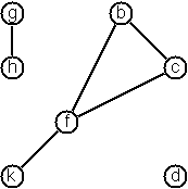
There are several ways to represent graphs in Prolog. One method is to represent each edge separately as one clause (fact). In this form, the graph depicted below is represented as the following predicate:
edge(h,g).
edge(k,f).
edge(f,b).
...
We call this edge-clause form. Obviously, isolated nodes cannot be represented. Another method is to represent the whole graph as one data object. According to the definition of the graph as a pair of two sets (nodes and edges), we may use the following Prolog term to represent the example graph:
graph([b,c,d,f,g,h,k],[e(b,c),e(b,f),e(c,f),e(f,k),e(g,h)])
We call this graph-term form. Note, that the lists are kept sorted, they are really sets, without duplicated elements. Each edge appears only once in the edge list; i.e. an edge from a node x to another node y is represented as e(x,y), the term e(y,x) is not present. The graph-term form is our default representation. In SWI-Prolog there are predefined predicates to work with sets.
A third representation method is to associate with each node the set of nodes that are adjacent to that node. We call this the adjacency-list form. In our example:
[n(b,[c,f]), n(c,[b,f]), n(d,[]), n(f,[b,c,k]), ...]
The representations we introduced so far are Prolog terms and therefore well suited for automated processing, but their syntax is not very user-friendly. Typing the terms by hand is cumbersome and error-prone. We can define a more compact and "human-friendly" notation as follows: A graph is represented by a list of atoms and terms of the type X-Y (i.e. functor '-' and arity 2). The atoms stand for isolated nodes, the X-Y terms describe edges. If an X appears as an endpoint of an edge, it is automatically defined as a node. Our example could be written as:
[b-c, f-c, g-h, d, f-b, k-f, h-g]
We call this the human-friendly form. As the example shows, the list does not have to be sorted and may even contain the same edge multiple times. Notice the isolated node d. (Actually, isolated nodes do not even have to be atoms in the Prolog sense, they can be compound terms, as in d(3.75,blue) instead of d in the example).
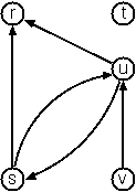
When the edges are directed we call them arcs. These are represented by ordered pairs. Such a graph is called directed graph. To represent a directed graph, the forms discussed above are slightly modified. The example graph above is represented as follows:
Arc-clause form
arc(s,u).
arc(u,r).
...
Graph-term form
digraph([r,s,t,u,v],[a(s,r),a(s,u),a(u,r),a(u,s),a(v,u)])
Adjacency-list form
[n(r,[]),n(s,[r,u]),n(t,[]),n(u,[r]),n(v,[u])]
Note that the adjacency-list does not have the information on whether it is a graph or a digraph.
Human-friendly form
[s > r, t, u > r, s > u, u > s, v > u]
Finally, graphs and digraphs may have additional information attached to nodes and edges (arcs). For the nodes, this is no problem, as we can easily replace the single character identifiers with arbitrary compound terms, such as city('London',4711). On the other hand, for edges we have to extend our notation. Graphs with additional information attached to edges are called labelled graphs.
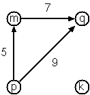
Arc-clause form
arc(m,q,7).
arc(p,q,9).
arc(p,m,5).
Graph-term form
digraph([k,m,p,q],[a(m,p,7),a(p,m,5),a(p,q,9)])
Adjacency-list form
[n(k,[]),n(m,[q/7]),n(p,[m/5,q/9]),n(q,[])]
Notice how the edge information has been packed into a term with functor '/' and arity 2, together with the corresponding node.
Human-friendly form
[p>q/9, m>q/7, k, p>m/5]
The notation for labelled graphs can also be used for so-called multi-graphs, where more than one edge (or arc) are allowed between two given nodes.
Problem 80
Write predicates to convert between the different graph representations. With these predicates, all representations are equivalent; i.e. for the following problems you can always pick freely the most convenient form. The reason this problem is rated (***) is not because it's particularly difficult, but because it's a lot of work to deal with all the special cases.
Example in Haskell:
λ> graphToAdj Graph ['b','c','d','f','g','h','k'] [('b','c'),('b','f'),('c','f'),('f','k'),('g','h')]
Adj [('b', "cf"), ('c', "bf"), ('d', ""), ('f', "bck"), ('g', "h"), ('h', "g"), ('k', "f")]
Problem 81
Write a function that, given two nodes a and b in a graph, returns all the acyclic paths from a to b.
Example in Haskell:
λ> paths 1 4 [(1,2),(2,3),(1,3),(3,4),(4,2),(5,6)]
[[1,2,3,4],[1,3,4]]
λ> paths 2 6 [(1,2),(2,3),(1,3),(3,4),(4,2),(5,6)]
[]
Problem 82
Write a predicate cycle(G,A,P) to find a closed path (cycle) P starting at a given node A in the graph G. The predicate should return all cycles via backtracking.
Example in Haskell:
λ> cycle 2 [(1,2),(2,3),(1,3),(3,4),(4,2),(5,6)]
[[2,3,4,2]]
λ> cycle 1 [(1,2),(2,3),(1,3),(3,4),(4,2),(5,6)]
[]
Problem 83
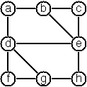
Write a predicate s_tree(Graph,Tree) to construct (by backtracking) all spanning trees of a given graph. With this predicate, find out how many spanning trees there are for the graph depicted to the left. The data of this example graph can be found in the file p83.dat. When you have a correct solution for the s_tree/2 predicate, use it to define two other useful predicates: is_tree(Graph) and is_connected(Graph). Both are five-minutes tasks!
Example in Haskell:
λ> length $ spanningTree k4
16
Problem 84
Write a predicate ms_tree(Graph,Tree,Sum) to construct the minimal spanning tree of a given labelled graph. Hint: Use the algorithm of Prim. A small modification of the solution of P83 does the trick. The data of the example graph to the right can be found in the file p84.dat.
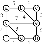
Example in Haskell:
λ> prim [1,2,3,4,5] [(1,2,12),(1,3,34),(1,5,78),(2,4,55),(2,5,32),(3,4,61),(3,5,44),(4,5,93)]
[(1,2,12),(1,3,34),(2,4,55),(2,5,32)]
Problem 85
Two graphs G1(N1,E1) and G2(N2,E2) are isomorphic if there is a bijection f: N1 -> N2 such that for any nodes X,Y of N1, X and Y are adjacent if and only if f(X) and f(Y) are adjacent.
Write a predicate that determines whether two graphs are isomorphic. Hint: Use an open-ended list to represent the function f.
Example in Haskell:
λ> graphG1 = [1,2,3,4,5,6,7,8] [(1,5),(1,6),(1,7),(2,5),(2,6),(2,8),(3,5),(3,7),(3,8),(4,6),(4,7),(4,8)]
λ> graphH1 = [1,2,3,4,5,6,7,8] [(1,2),(1,4),(1,5),(6,2),(6,5),(6,7),(8,4),(8,5),(8,7),(3,2),(3,4),(3,7)]
λ> iso graphG1 graphH1
True
Problem 86
a) Write a predicate degree(Graph,Node,Deg) that determines the degree of a given node.
b) Write a predicate that generates a list of all nodes of a graph sorted according to decreasing degree.
c) Use Welch-Powell's algorithm to paint the nodes of a graph in such a way that adjacent nodes have different colors.
Example in Haskell:
λ> kColor ['a','b','c','d','e','f','g','h','i','j'] [('a','b'),('a','e'),('a','f'),('b','c'),('b','g'),('c','d'),('c','h'),('d','e'),('d','i'),('e','j'),('f','h'),('f','i'),('g','i'),('g','j'),('h','j')]
[('a',1),('b',2),('c',1),('d',2),('e',3),('f',2),('g',1),('h',3),('i',3),('j',2)]
Problem 87
Write a predicate that generates a depth-first order graph traversal sequence. The starting point should be specified, and the output should be a list of nodes that are reachable from this starting point (in depth-first order).
Example in Haskell:
λ> depthFirst ([1,2,3,4,5,6,7], [(1,2),(2,3),(1,4),(3,4),(5,2),(5,4),(6,7)]) 1
[1,2,3,4,5]
Problem 88
Write a predicate that splits a graph into its connected components.
Example in Haskell:
λ> connectedComponents ([1,2,3,4,5,6,7], [(1,2),(2,3),(1,4),(3,4),(5,2),(5,4),(6,7)])
[[1,2,3,4,5][6,7]]
Problem 89
Write a predicate that finds out whether a given graph is bipartite.
Example in Haskell:
λ> bipartite ([1,2,3,4,5],[(1,2),(2,3),(1,4),(3,4),(5,2),(5,4)])
True
λ> bipartite ([1,2,3,4,5],[(1,2),(2,3),(1,4),(3,4),(5,2),(5,4),(1,3)])
False